Basic Analyses

Additional Information on Regression Analysis

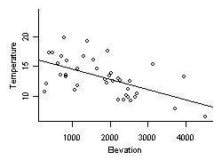
Regression analysis is a method for estimating a relationship of a specified functional form between a response variable and one or more explanatory variables. Common examples of regression relationships in stream ecosystems include modeling biological characteristics (e.g., species richness) as a function of different environmental factors, or modeling local environmental condition (e.g., stream temperature) as a function of other data that can be extracted from maps.

The most common functional form that is assumed for a regression analysis is a linear relationship:

where E(y) denotes the expected value for the variable y, b_iare constant coefficients, x_iare different explanatory variables, and n is the number of explanatory variables. Here, as in all regression analysis, it is assumed that the response variable is measured with some inherent error, or sampling variability, and regression analysis is used to estimate the relationship between the explanatory variables and the mean, or expected value of y.

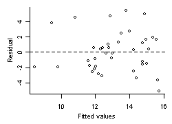
Regression analysis can be used to fit relationships between any variables with little consideration of the underlying assumptions. However, when the estimated relationships are used to predict likely values of y at new values of the explanatory variables, or when the estimated relationships are interpreted with respect to whether they accurately represent the underlying physical or biological relationships, the theoretical assumptions must be considered more carefully. More specifically, one must assess whether the assumed functional form is sufficiently representative of the actual relationship, whether the sampling variability in y is distributed as assumed, whether the magnitude of the sampling variability in y changes across the range of predictions, whether the samples used to fit the model are independent, and whether errors in the measured values of the explanatory variables are small enough to be ignored. We discuss each of these assumptions in more detail and illustrate methods for assessing the degree to which assumptions are supported by the data.

Is the Assumed Functional Form Appropriate?

Figure 1. Stream temperature vs. elevation in Oregon. Solid line is a simple linear regression fit to the data. — **Figure 1**. Stream temperature vs. elevation in Oregon. Solid line is a simple linear regression fit to the data.

A frequent assumption of regression analysis is that relationships are linear with respect to the explanatory variables. For example, average summer daytime stream temperatures in Oregon appear to decrease linearly with increased elevation (Figure 1). In many cases, linear relationships provide a reasonably accurate estimate of the underlying relationships, especially when there are no reasons for assuming differently. Ecological knowledge of the underlying processes can often provide guidance as to the appropriate functional form. For example, an appropriate functional form for a model relating the abundance of a species to environmental factors would likely be unimodal, as the abundances of different species are thought to be highest at some optimal value of each environmental gradient, and decrease on either side of this optimum point.

Is the Assumed Distribution for Sampling Variability Appropriate?

Regression analysis seeks to find a relationship between the expected, mean value of the response variable, y, and different explanatory variables. A key assumption for accurately estimating this relationship is the distribution of the error, or variability, in observed values of y. The most common assumption is that sampling error in y is normally distributed. That is, for any combination of explanatory variables, we assume that the scatter of observed values about the mean follows a normal distribution.

Figure 2. Quantile-quantile plot comparing residuals from regression fit shown in Figure 1 with a normal distribution. — **Figure 2**. Quantile-quantile plot comparing residuals from regression fit shown in Figure 1 with a normal distribution.

One way to assess whether this assumption holds true for a particular data set is to compare the distribution of residual values with a normal distribution. Residual values are defined as the difference between the modeled mean value and the observed value, and overall, these values should be normally distributed. Q-Q plots provide a robust, graphical approach for assessing whether residuals are normally distributed. In the example shown in Figure 2 for Oregon stream temperature, most values cluster around the solid line, indicating a near-normal distribution. However, deviations at the upper and lower end suggest that slight deviations from normality may exist. More egregious departures from normality would indicate that data are not close enough to normal to model effectively with this assumption.

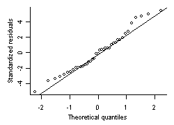
In assessing the assumption of normal sampling variability, it is often useful to consider the characteristics of the response variable. Many typical response variables are constrained and by definition, sampling variability is not normal. For example, variables that measure a count (e.g., total taxon richness) have a minimum value of 0, and those that measure a proportion (e.g., relative abundance) have a minimum value of 0 and a maximum value of 1. In general, normal distributions do not allow for such constraints, and therefore, may not be appropriate. However, some variables may appear to be constrained (e.g., multimetric indices) but are reasonably well approximated by a normal distribution. Other variables that have a minimum value of zero (e.g., chemical concentrations, watershed area) are normally distributed after a log transformation. Generalized linear models also allow one to directly model certain types of data with non-normal distributions.

Is the Sampling Variance Constant?

Figure 3. Residuals vs. fitted values for regression fit shown in Figure 1. — **Figure 3**. Residuals vs. fitted values for regression fit shown in Figure 1.

When sampling variability is assumed to be normally distributed, the magnitude of this variability is estimated from the variance of the residuals (Figure 3). The accuracy of this estimate depends strongly on an assumption that the magnitude of sampling variability is constant for all predicted values. A straightforward method for testing this assumption is to plot residual values against fitted values, and assess whether the scatter of the residual values is constant over the entire range of fitted values. In our example of Oregon temperature, this assumption seems reasonably well supported by the distribution of residuals. Other common phenomenona include residual variance that increases with increases in fitted values (e.g., trumpet-shaped plots), which would suggest that sampling variance is not constant, and prediction intervals are not likely to be accurate.

Are Samples Independent?

Regression models typically assume that samples are independent from one another, and when this assumption is violated, more confidence may be ascribed to results than is supported by the data. Considerations of whether samples are independent are covered in depth on the Autocorrelation page.